La spécificité du tadalafil est liée à sa longue demi-vie, permettant une action qui excède largement celle des autres inhibiteurs de PDE5. L’absorption digestive est complète, avec un pic plasmatique atteint en 2 heures environ. Le métabolisme est réalisé via CYP3A4, produisant des métabolites inactifs éliminés principalement dans les fèces. La sélectivité enzymatique est élevée, réduisant les effets indésirables extra-caverneux. Les réactions indésirables fréquentes incluent céphalées, bouffées vasomotrices et troubles digestifs légers. L’activité pharmacologique est stable, indépendamment de l’ingestion d’aliments. Dans les comparaisons de longue durée, acheter cialis pas cher est mentionné en relation avec les études portant sur la persistance d’efficacité et la constance de la cinétique plasmatique.
Navneuronet.narod.ru
Kalman extension of the genetic algorithm
Los Alamos National Laboratory, MS-F607, Los Alamos, NM 87545
LAUR-00-150, SPIE proc. vol. 4055, April, 2000
ABSTRACT
In typical GA application, the fitness assigned to a chromosome-represented individual in the context of a specified
environment takes a deterministic calculable value. In many problems of interest, the fitness of an individual is stochastic,
and the environment changes in unpredictable ways. These two factors contribute to an uncertainty that can be associated
with the estimated fitness of the individual.
The Kalman formulation provides a mechanism for a useful treatment of uncertainty within the GA framework. It provides
for tracking the best-estimated fitness, and for assessing the uncertainty of the best-estimated fitness. The stochastic
uncertainty of an existing individual can be reduced by additional evaluation of the fitness. The process (environmental)
noise causes an increase in uncertainty as the age of the last evaluation increases. In a Kalman-extended genetic algorithm,
we want to know the value of re-evaluating an existing solution in the population relative to generating and evaluating new
individuals. A scheme for efficient allocation of computational resources among existing individuals and new individuals is
This Kalman-Darwin formulation is applied to the problem of maintaining an optimal network configuration of links between
moving nodes, with time-dependent, stochastic blockages. The nodes, for example, could be environmental sensors with
radio transmitter/relays located on vehicles, and the network is configured to provide communication paths from each sensor
back to a central node with minimum message loss. As the sensors move, the optimal network changes, but information
contained within the GA population of solutions allows new optima to be efficiently obtained. The performance of this
approach is explored and results are presented. 1. INTRODUCTION
The Kalman Genetic Algorithm (KGA) is an extension of the genetic algorithm (GA)1-3 in which Kalman filtering4-6 is
applied to the fitness values associated with the population of chromosomes. In the GA, a chromosome represents a trial
solution to a problem. The chromosome has a well-defined measure of fitness within the context of the problem space or
environment. In many interesting applications, the environment is dynamic. The fitness of a given chromosome will change
in time, as changes occur in the environment. In addition, for environments of sufficient complexity, or for environments
with stochastic elements, the fitness of a chromosome is unknowable, and can only be approximated. The Kalman
formulation provides a natural mechanism for extending the domain of application of the genetic algorithm from static,
prescribed problem spaces to dynamic, and complex or stochastic environments.
In the KGA, at any given time, each chromosome has a best-estimated fitness and an uncertainty associated with that
estimate. The fitness and uncertainty are updated according to the Kalman formulation, as the environment changes with the
* Correspondence: E-mail: [email protected]; Telephone: 505-667-6654
passage of time, and when a chromosome is re-evaluated. Knowledge is acquired7 by re-evaluating an existing trial solution
(thereby decreasing the uncertainty associated with its fitness estimate) or by generating and evaluating a new trial solution.
The principle behind the KGA is simple. The population, consisting of N individuals, each with a best-estimated fitness, can
be characterized by the variance V of these N fitness values. When the uncertainty associated with all members of the
population is smaller than V, the population is treated as sufficiently evaluated, and the algorithm will generate and evaluate
a new trial solution. However, if any of individuals in the population have uncertainties greater than V, the algorithm will re-
evaluate whichever individual has the highest uncertainty.
The literature contains applications in which GA is used to tune the parameters of a Kalman filter.8-11 There is also some
research reported as a hybridization of Kalman filtering and GA, in which Kalman filtering and GA are used to optimize two
separate parts of a problem.12,13 In previous work,14-17 the author used GA to periodically optimize controllers in the context
of a dynamic environment. The heuristic of including the previous best solution in the next initial population was explored,
but a theoretical formulation underlying the use of GA in noisy, dynamic environments was lacking. In a SciSearch® search
of 17.5 million technical articles, no reference was found in which a Kalman filter is used as an integral part of the GA
2. MECHANICS OF THE KALMAN GENETIC ALGORITHM
The KGA keeps a population of individuals. An individual represents a trial solution to a problem. There is an upper limit, N,
on the population size, and at any given time, there are actually n individuals in the population. The individual, i, has four
elements: 1) a chromosome W , 2) a best estimated fitness, f , 3) an uncertainty, P , associated with that estimate, and 4) a
timestamp, T , specifying the time that the uncertainty was last updated. The chromosomes can take a variety of forms.18 The
requirements on the form of the chromosome are that it can be transformed into a possible solution of the problem, and that a
set of genetic operators can be constructed for it. For this implementation, the chromosomes are simply fixed length
sequences of bounded integers. A mechanism for transformation from the chromosomal form (the genotype) to the problem
solution form (the phenotype) must be developed for each problem. As an aid to interpretation of the uncertainty, the
underlying fitness can thought of as the best estimate of fitness, plus or minus the square root of the uncertainty.
When a real-time directed-search algorithm is used in a dynamic environment, the algorithm computational time is
interwoven with the physical time. We consider the case in which an evaluation of the fitness of a trial solution takes a finite
amount of time, τ . During a given period of time, there will thus be a finite number of trial evaluations that the algorithm
A mechanism is required to evaluate the fitness of a solution. In environments with stochastic processes, the result of a fitness
evaluation will be a real-number value that represents the true, underlying fitness value but has an uncertainty associated with
it. If an ensemble of fitness evaluations were to be made on a trial solution, the variance of the ensemble of the resulting
fitness values, R, is taken as the measure of the uncertainty in the fitness evaluation. This variance is analogous to the
observation noise variance of the Kalman formulation, if a fitness evaluation is treated like an observation. R can be
interpreted as the uncertainty with which the result of a fitness evaluation represents the true, underlying fitness of the trial
solution. R designates the variance of the observation noise associated with a single evaluation of a trial solution.
Because the environment is dynamic, the underlying fitness of a given trial solution will change with time. In the Kalman
formulation, this change is attributed to process noise. Like the observation noise, the process noise is characterized by a
variance, in this case designated by Q. Q gives the variance in the change in the underlying fitness of trial solutions during a
specified time interval, due to change in the environment. In this formulation, there is no fixed time interval to use to define
Q, as is common in Kalman filtering applications. Instead, a “process noise rate”, given by q, is used. The process noise
variance expected after the environment undergoes changes for a time interval dt, is Q = dt q. This presumes that the process
noise variance increases linearly with time interval, although alternative formulations could be used as well. As with any
Kalman application, q can be specified by knowledge about the environment, or it can be evaluated adaptively.
The KGA begins operating at time t = t . At this time, the population contains no trials yet (n = 0). The algorithm iterates over
four main processes, as shown schematically in Fig. 1. The first process updates the uncertainties of the members of the
population to the current time. If an uncertainty was last updated at time T , the associated uncertainty increases according to
This is analogous to the Kalman equation that updates the covariance matrix for process noise. The time of the last update is
then advanced to the current time, T = t.
Figure 1. The Kalman-extended genetic algorithm, shown schematically as a cycle over four major processes.
The second process characterizes some statistics of the population that will determine whether to generate a new trial, or re-
evaluate an existing individual. The variance, V, of the best-estimated fitnesses of the individuals in the population is
, of the most uncertain individual. These two statistics are used by the
algorithm to determine which of the three elements of the third process to invoke.
The third process performs a fitness evaluation. There are three alternatives for this third process. If the population is not full
(i.e. n<N), a new random chromosome is generated and evaluated. The second alternative for the evaluation process: if the
population is full, and the uncertainty of the most uncertain individual exceeds the population’s fitness variance (i.e. P
the most uncertain individual will be reevaluated. When a re-evaluation is performed (returning a value of g), the previous
, is updated using the Kalman observation equation:
In addition, a re-evaluation reduces the uncertainty P by multiplying by a factor of R/(P+R) as follows:
The quantity P/(P+R) is analogous to the gain, K, of the Kalman formulation.
The third alternative for the evaluation process: if the population is full, and the uncertainty of the most uncertain individual
is less than the population’s fitness variance, a new trial will be generated and evaluated. Traditional GA mechanics are used
to generate new individuals. Two parents are selected based on their fitness, with more fit individuals being more likely to be
selected. Genetic operators such as crossover and mutation are used to generate a new chromosome from those of the parents.
When a new chromosome is created and evaluated once, the best estimate of fitness f is the result of the evaluation, and the
The fourth process incorporates the newly evaluated trial appropriately into the population. The best-estimated fitness and the
uncertainty are combined to give an uncertainty-compensated fitness, F, for each individual, given by
The algorithm thus searches for individuals with high fitness, but discounts the fitness if there is a high associated
uncertainty. The population is sorted by this uncertainty-compensated fitness. If the uncertainty-compensated fitness of the
new chromosome is better than that of the least fit individual in the population, the new individual is added to the population,
and the least fit individual is discarded. If the population is not yet full, or if an existing individual was reevaluated, the
population is simply re-sorted according to uncertainty-compensated fitness. At any time, the individual with the best
uncertainty-compensated fitness is taken to be the best-adapted solution produced by the algorithm. These four processes
take some time to perform, but the bulk of the time is presumably spent evaluating trials. When the cycle repeats, the time t is
3. DEVELOPMENTAL TEST-BED: NETWORK CONFIGURATION OPTIMIZATION
A test-bed has been constructed for developing and experimenting with the KGA in a simulated dynamic, noisy environment.
It has been implemented in Java, with a GUI that allows a user to easily construct scenarios and observe simulations of the
The test problem is to configure a network of radio links connecting a set of nodes to a collection point. The task is to
maintain a good configuration of links as the nodes move. This test application derives from a system of atmospheric aerosol
sensors mounted on vehicles, which deliver their data via radio links to a collection point. Each sensor collects a stream of
data, which it then transmits via a low-power radio link. A sensor node may transmit directly to the collection point or to
another node. A node can receive and repeat data from other sensors. The network of links thus is an acyclic, directed graph
(i.e. a tree) with the base being the collection point, and the sensors forming the other nodes. Each radio link forms an edge of
In its pure, unconstrained form, this problem admits an algorithmic solution (via Dijkstra’s shortest-path tree algorithm).19-21
The existence of this solution does not render the application trivial, because slight variations in the problem definition, as
would be encountered in practice, make this problem NP-complete.19 Examples of such variations include: a constraint on
the number of links a given node may receive and retransmit; a bandwidth limitation on the transmission channels or a
degradation in transmission fraction with increased message traffic; a maximum number of links in a path to the collection
point; or the possibility of redundant paths, where a node may transmit to more than one receiver. Optimization of a complex
network with routing and bandwidth constraints is not amenable to algorithmic approaches, but can be attacked with GA.22
The existence of an algorithmic solution for the pure form of the problem does allow the performance of the KGA to be
assessed relative to the sequence of optimal solutions.
The nodes are treated as executing a random walk within a prescribed area. (The vehicles are not dedicated to the sensors, but
are engaged in other activities.) The movement of the nodes makes the problem environment dynamic. As the nodes move,
the transmission probability along the links changes, and the optimal network configuration also changes.
A prescribed area on the ground of arbitrary shape and size is represented on a 2D Cartesian cell grid. The cell size, and the
number of cells spanning the two dimensions, are adjustable. A baseline scenario has been constructed, in which each cell
represents a 160 by 160 meter square, and a grid of 125 by 125 cells covers a 20 by 20 km area. In this baseline scenario, the
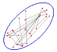
vehicle/sensor/nodes are restricted to a roughly 10 by 20 km elliptical region as shown in Fig 2.
Figure 2. Example scenario, showing a user-prescribed region, 25 randomly placed nodes, and a randomly generated link network. The
collection point is shown as the open circle.
Let S designate the total number of nodes, exclusive of the collection point. The baseline scenario contains 25 sensor nodes.
These vehicle-mounted sensors can be initialized by assigning each sensor to a random cell within the prescribed area. Only
one sensor can occupy a cell. Fig. 2 shows the locations of 25 randomly placed sensors.
Each node establishes a radio link to another node or to the collection point, to transmit its own data, and any data it receives
from other nodes. Each node has a unique ID in the range of one to S. The receiver of a node is specified by an integer in the
range of zero to S. A value of zero indicates that the link is transmitting directly to the collection point, while any other value
specifies the ID of the receiving node. The network configuration is completely specified by giving the receiver for each
node.19 This requires a total of S integers, each in the range 0 to S. A node can not have itself as a receiver. The number of
distinct network configurations is then SS. For 25 sensors, there are 8.9(10)34 possible network configurations.
In this implementation, only valid spanning-trees configurations (including the collection point) are considered, i.e. all nodes
and the collection point are included in the graph, and there are no cyclic paths in the graph. This reduces the size of the
problem space. A simple algorithm is used to generate random trees, as follows. All nodes are initially unconnected. An
unconnected node is selected at random. A receiver is selected at random from the set containing the collection point and all
connected nodes. The selected unconnected node takes the randomly selected receiver to be its receiver, and then becomes a
connected node. This process is repeated until all nodes are connected. A randomly generated network linking 25 sensors to a
collection point is shown in Fig. 2. The 25 integer representation of this network is { 8 19 17 18 12 20 20 20 11 0 21 0 20 20
13 12 12 20 24 12 0 6 18 12 21}. Node 1 transmits to node 8, while nodes 10, 12 and 21 transmit to the collection point, etc.
The expected transmission fraction over a link depends on the length of the link. For short distances, the expected
transmission is nearly perfect, because the signal is much higher than the noise. There is a scale distance, d, where the
expected transmission fraction across a link is reduced to one half; for significantly longer transmission distances, the
transmission fraction will be very small (extinction and the 1/r2 antenna gain relation degrades the signal, which becomes
obscured in noise.) There is another scale distance, w, which characterizes the distance over which the transmission fraction
drops from near one to near zero. A parameterized formulation is used for the transmission fraction from node i to node j:
where d designates the distance from node i to node j. The transmission as a function of distance is shown in Fig. 3 for d =
5000 m and w = 100 m. If the path from a node to the collection point contains a sequence of links, the total transmission
fraction from the node to the collection point is simply the product of the transmission fractions of each link in the path.
Fig. 3. The transmission fraction across a link, as a function of the length of the link, using the parameterized formulation with d=5000 m,
The fitness of a network configuration can be characterized in a variety of ways, depending on what is important in any given
application. For the test-bed application, the network configuration fitness is simply the average, over all nodes, of the
transmission loss from each node to the collection point. The goal of maximizing transmission fraction is then equivalent to a
goal of minimizing message transmission loss. For the random network shown in Fig. 2, the average message loss is 0.94594.
The shortest-path algorithm was used to generate the network that minimizes the transmission losses from each node to the
collection point. The shortest-path tree algorithm minimizes the sum of the weights associated with all edges in the paths
from any node to the root node. The algorithm can be used by equating the weight associated with an edge to the natural log
of the inverse of the transmission fraction. Then minimizing the sum of the weights along a path is equivalent to maximizing
the total transmission fraction along the path. The shortest-path network is shown in Fig 4, where the sensors have the same
locations as in Fig. 2. For this network configuration, the average message loss fraction is 0.03185, which is representative of
25 sensors in a 10 by 20 km elliptical area, where the transmission range scale is 5 km.
Fig. 4. The shortest-path tree for 25 randomly located nodes.
The dynamic environment is implemented as follows. A simulation is run in which the time is advanced in steps of durationτ . During each time step, the fitness of one network configuration is evaluated, as prescribed by the KGA. In addition, during
each time step, a sensor may move, causing a change in the environment. In order to explore sensitivity of the KGA to
process noise, the expected change in fitness during a time step can be varied by controlling how often sensors are moved.
The process noise rate is then calculated adaptively, using a fixed-gain recursive filter and the observed fitness changes
caused by the sensor movements. If, for example, sensors are moved (to one of the eight nearest-neighbor cell locations) at a
rate of one movement per 500 time steps, the process noise variance is found to average approximately 8.51E-11 in a time
step. During the 100 time steps which would be required to re-evaluate all members of a 100-member population, the process
noise would be ~10E-8, corresponding to a typical fitness change of ~0.0001. This process noise level is about one part in
300 of typical near-optimal network configurations in the baseline scenario. In a simulation starting with the sensor
configuration shown in fig. 2 and incurring 500 sensor movements, the fitness of the shortest-path tree network configuration
varies over the range of 0.0295 to 0.0335. If the links in the initial shortest-path network configuration were left unchanged
during these 500 sensor movements, the fitness would be significantly degraded.
The observation noise, R, is implemented as follows. The transmission fraction over a link depends not only on the length of
the link, but also on stochastic factors such as the atmospheric conditions and line-of-sight obstructions. These stochastic
factors contribute to the observation noise that gives variation in the actual fitness of a network configuration. In the test-bed,
process noise is added to average transmission fraction of a network configuration whenever it is evaluated. An evaluation of
the fitness of a given network configuration for a given set of node positions is artificially given an error, by adding
(2r-1)sqrt(3R), where r is a random number between 0 and 1. This produces a distribution of observation noise with a
An implementation of the genetic algorithm is used which takes a sequence of integers as its chromosome, where the integers
are bounded in zero to a specified maximum value. In this case, the chromosome has S integers, each in the range of [0, S].
The population size is 100 individuals. The first 100 individuals are created as random tree configurations. When the
algorithm determines that a new trial solution should be generated, two parents are selected. This selection is based on fitness
rank, with the most fit individual being 2.5 times more likely to be selected than the median fit individual. Generation of new
individuals uses two-point cross-over, followed by mutation and a repair step. The cross-over causes complete genes (i.e.
integers in 0 to S) to be taken from the parents into the child: there is no splitting of genes. The mutation step selects two
genes at random, and resets them to new random values, corresponding to a receiver node selected at random from those
connected to the collection point. The repair step ensures that the resulting network configuration is an acyclic spanning tree
rooted on the collection point. Every gene that is part of a valid tree is retained – those that are not are replaced with alleles
that correspond to a link to a connected node. If the algorithm determines that an existing individual should be re-evaluated,
4. RESULTS
A simulation was run in which the observation noise variance, R, of the fitness (the message loss fraction) was set to 1E-8.
Since the message loss fraction of good configurations is around 0.03, the standard deviation of the observation noise of 1E-4
is about one part in 300, which can be considered to be a low level of observation noise. For this case, the process noise
variance is approximately 8.51E-11 per time step, which is achieved by moving the sensors at the rate of one movement per
500 time steps. As described above, for a population size of 100, this process noise standard deviation is below one part in
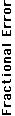
300, which can be considered to be a low level of process noise. Fig 5 shows the fractional error of the actual fitness (average
message loss rate, with observation noise removed) of the best member (lowest uncertainty-compensated message loss
fraction) of the population relative to the fitness of the shortest-path network configuration, i.e. (f-f )/f . Initially, when the
KGA has evaluated only one random configuration (that shown in Fig. 2) the loss of the best configuration is 0.94594, while
the loss with the optimal configuration is 0.03185, so the fractional error of the KGA relative to optimal has a high initial
value of 2870%. As the KGA generates and evolves its population of trial solutions, the fractional error is seen to drop. After
about 20,000 trial evaluations, the best solution in the KGA population is within 0.1% of the optimal solution. In this case,
the KGA often attains the optimal solution.
During the 250,000 time steps of the simulated run, the KGA evaluated 100 random configurations, generated and evaluated
55,674 new configurations, and re-evaluated existing configurations 194,226 times. When the observation noise is low, the
algorithm spends 22% of its resources on new trial solutions, and 78% on re-evaluating existing solutions. Note that once a
population has converged somewhat on the optimal configuration, when a new trial is generated, it will have a larger
uncertainty than the bulk of the population. If the fitness of the new trial is good enough to earn it a place in the population,
the algorithm will then re-evaluate the new trial until its uncertainty drops below the population variance.
Several events can be seen in fig. 5 as spikes in the fractional error. These occur when the motion of the sensors causes the
optimal network configuration to undergo a significant restructuring. The fractional error between the best KGA solution and
the optimal solution may rise to a few percent on these occasions, but then drops back down as the KGA discovers the new
configuration. Note that these recoveries require one or two thousand time steps, compared to the 20,000 time steps required
to reach near-optimal solutions beginning from scratch. Number of Evaluations
Fig. 5. The fractional error of the message loss fraction of the best KGA solution relative to that of the optimal network configuration,
showing how closely the KGA tracks the optimal network configuration. There is one trial evaluation per time step. The process noise
variance is approximately 10E-10 per timestep, and observation noise variance is 10E-8, for 25 sensor network starting from the locations
shown in Fig. 2. The loss fraction of the optimal configuration ranges from 0.0295 to 0.0334.
A second case was run in which the process noise was increased by a factor of about 100. This was accomplished by moving
the sensors at a rate of one sensor motion every 50 time steps, which results in a process noise variance that averaged 9.26E-9
per time step. This corresponds to a process noise standard deviation of about 0.001 in 100 time steps (one for each member
of the population), which is about 3% of the fitness of near-optimal configurations. As shown in fig. 6, this increased process
noise degrades the ability of the KGA to track the optimal network configuration. Where the optimal configuration has a
message transmission fraction that varies from 0.0264 to 0.0357, with an average value of 0.02978 (excluding the first 20,000
time steps), the KGA has an average message loss fraction of 0.03093 during the same period. On average the KGA solution
is 3.9% worse than the optimal configuration, excluding the first 20,000 time steps, at this process niose level of 3%. For this
case, there is little change in the resource allocation between re-evaluation and new trial generation: the KGA called for new
trial solutions in 21.1% of time steps.
A third case was run which was the same as the first, except that the observation noise variance was increased by a factor of
100, to a moderate level of 1.E-6. The process noise remained at the low level of 1E-10 per time step. The observation niose
standard deviation (0.001) is about 3% of the fitness of near-optimal configurations for this third case. Fig. 7 shows how the
KGA is able to track the optimal configuration at this noise level. After an initial period of 20,000 time steps, the KGA
configuration is on average 1.92% worse than the optimal configuration. At this observation noise level, significantly more
resources are allocated to re-evaluation of existing trials: new trial configurations are generated and evaluated in only 8.1% of
Number of Evaluations
Fig. 6. The fractional error of the message loss fraction of the best KGA solution relative to that of the optimal network configuration. The
case is identical to that shown in Fig 5, except that the process noise variance is increased by a factor of 100 to a value of approximately
Number of Evaluations
Fig. 7. The fractional error of the message loss fraction of the best KGA solution relative to that of the optimal network configuration. The
case is identical to that shown in Fig 5, except that the observation noise variance, R, is increased by a factor of 100 to a value of
5. CONCLUSIONS
The overall conclusion of this work is that the Kalman formulation can be integrated into the genetic algorithm formulation
in a compelling way to create a Kalman-extended genetic algorithm that can perform ongoing directed searches in dynamic,
noisy environments. The extension of a population of individuals, each with a fitness, by associating an uncertainty with the
fitness of each individual, is conceptually clear, and easy to implement. The mechanics of updating the best-estimated fitness
and the uncertainty after a re-evaluation follow directly from the Kalman formulation. The very simple implementation of the
KGA, where a new trial is generated and evaluated whenever the uncertainty of the most uncertain individual is less than the
variance of the population fitnesses, has been found to work, through experimentation in a test-bed.
The KGA can be viewed as a mechanism to allocate resources between the two complimentary activities of re-evaluating
existing solutions for changing conditions, and generating new solutions. The allocation depends on the level of observation
noise: the more uncertain the observations are, the more resources must be dedicated to re-evaluation of existing solutions.
Even when observation noise is low, however, a somewhat surprising result is that only 21 or 22% of effort should be
expended on new solutions, while the remainder should go to re-evaluating existing solutions.
At low levels of process and observation noise (±0.3%), the KGA was shown to be able to maintain near-optimal solutions.
At moderate observation noise level (±3%), the KGA was still able to maintain configurations with fitness values within an
average of 2% of the optimal configuration. At moderate process noise level (±3%), the KGA was able to maintain
configurations with fitness values within an average of 4% of the optimal configuration.
In contrast to the traditional GA wherein a bigger population is better, in the KGA there is an optimal population size. If the
population were too large, the KGA would waste time evaluating relatively poor individuals that have grown obsolete (i.e.
whose uncertainty has increased too much). There are indications that the optimal population size can be re-evaluated on an
ongoing basis, using R, q τ , and V.
The formulation presented here was developed with simplicity as a criterion. Alternative forms may be more effective. For
example, the uncertainty-compensated fitness, which is used to rank the individuals in the population, could be a more
complex function of the best-estimated fitness, the uncertainty, and/or the square root of the uncertainty. The criteria for
selecting which individual to evaluate next could depend on the best-estimated fitness in addition to the uncertainty. The
population fitness variance could also be formulated differently.
When a new trial is generated and evaluated, its uncertainty is generally much higher than that of the existing individuals.
The new trial should therefore be re-evaluated several times to reduce its uncertainty to a level at which a valid comparison
can be made to the existing individuals. Less fit trials can be discarded at higher level of uncertainty, improving the
efficiency of the algorithm. This is an avenue for improvement of the formulation presented here, in which a new trial is
compared with the population after only a single fitness evaluation. REFERENCES
J. H. Holland, Adaptation in Natural and Artificial Systems, MIT Press, Cambridge, MA (1992).
D. E. Goldberg, Genetic Algorithms in Search, Optimization and Machine Learning, Addison-Wesley Publishing Co.
David B. Fogel, Evolutionary Computation : Toward a New Philosophy of Machine Intelligence, IEEE Press (1995).
R. E. Kalman, “A new approach to linear filtering and prediction problems,” Trans. AMSA Journal of Basic
Engineering, vol. 82, pp 35-45 (1960).
R. E. Kalman and R. S Bucy, “New results in linear filtering and prediction theory,” Trans. AMSA Journal of Basic
Engineering, vol. 82, pp 95-108 (1961).
S. Haykin, “Adaptive filter theory,” Prentice-Hall Information and System Science Series (1986).
H. Plotkin, Darwin Machines and the Nature of Knowledge, Harvard University Press, Cambridge, MA (1994).
P. E. Howland, “Target tracking using television-based bistatic radar,” IEE Proc. Radar Sonar and Navigation, v.
M. J. Arcos, C. Alanso, and M. C. Ortiz, “Genetic-Algorithm-Based Potential Selection in Multivariant Voltammetric
Determination of Indomethacin and Acemethacin by Partial Least-squares, “ Electrochimica Acta, v. 43(#5-6) pp.
W. S. Chaer, R. H. Bishop, and J. Ghosh, “A Mixture-of-Experts Framework for Adaptive Kalman Filtering,” IEEE
trans. On Systems, Man, and Cybernetics, Part B-Cybernetics , vol. 27, no. 3, pp. 452-464 (June 1997).
K. G. Berketis, S. K. Katsikas, and S. D. Likothanassis, “Multimodal Partitioning Filters and Genetic Algorithms,”
Nonlinear Analysis-Theory Methods & Applications, vol. 30, no. 4, pp. 2421-2427 (Dec 1997).
L. A. Wang, J. Yen, “Extracting Fuzzy Rules for System Modeling using a Hybrid of Genetic Algorithms and Kalman
Filter,” Fuzzy Sets and Systems, vol. 101, no. 3, pp. 353-362 (Feb 1, 1999).
S. E. Aumeier, J. H. Forsmann, “Evaluation of Kalman Filters and Genetic Algorithms for Delayed-Neutron
Nondestructive Assay Data Analyses,” Nuclear Technology, v. 122, no. 1, pp. 104-124 (April 1998).
Phillip D. Stroud, “Evolution of Cooperative Behavior in Simulation Agents,” SPIE proc. vol. 3390 (April 1998).
Phillip D. Stroud, “Adaptive Simulated Pilot,” Journal of Guidance, Control, and Dynamics, Eng. notes, vol. 21, no. 2,
Phillip D. Stroud, “Learning and Adaptation in an Airborne Laser Fire Controller,” IEEE Transactions on Neural
Networks, vol.8, no. 5, pp. 1078-1089 (Sept 1997).
Phillip D. Stroud, and Ray C. Gordon, “Automated Military Unit Identification in Battlefield Simulation,” SPIE proc.
Z. Michalewicz, “Genetic Algorithms + Data Structures = Evolution Programs,” 2nd ed., Springer, Berlin (1992).
L. J. Dowell, “Optimal Configuration of a Command and Control Network: Balancing Performance and
Reconfiguration Constraints,” Proceedings of the 2000 ACM Symposium on Applied Computing (March 2000).
E. W. Dijkstra, “A Note on Two Problems in Connexion with Graphs,” Numerische Mathematik 1, pp. 269-271
E. Minieka, “Optimization algorithms for networks and graphs,” M. Dekker, New York (1978).
King-Tim Ko, Kit-Sang Tang, Cheung-Yau Chan, Kim-Fung Man, Sam Kwong, “Using Genetic Algorithms to Design
Mesh Network,” Computer, Vol. 30, No. 8 (August 1997).
Smithers Summary Shandi Hopkins was admitted to the residential treatment program, Smithers Alcoholism and Rehabilitation Center, at Roosevelt Hospital on 4/18/01 and discharged 5/27/01. He was in touch with me regularly, sometimes twice a day while in the program. I obtained an 800 number to enable him to stay in touch with me when I moved from New York last July to begin teaching at Illinoi
 (i.e. a tree) with the base being the collection point, and the sensors forming the other nodes. Each radio link forms an edge of
In its pure, unconstrained form, this problem admits an algorithmic solution (via Dijkstra’s shortest-path tree algorithm).19-21
The existence of this solution does not render the application trivial, because slight variations in the problem definition, as
would be encountered in practice, make this problem NP-complete.19 Examples of such variations include: a constraint on
the number of links a given node may receive and retransmit; a bandwidth limitation on the transmission channels or a
degradation in transmission fraction with increased message traffic; a maximum number of links in a path to the collection
point; or the possibility of redundant paths, where a node may transmit to more than one receiver. Optimization of a complex
network with routing and bandwidth constraints is not amenable to algorithmic approaches, but can be attacked with GA.22
The existence of an algorithmic solution for the pure form of the problem does allow the performance of the KGA to be
assessed relative to the sequence of optimal solutions.
(i.e. a tree) with the base being the collection point, and the sensors forming the other nodes. Each radio link forms an edge of
In its pure, unconstrained form, this problem admits an algorithmic solution (via Dijkstra’s shortest-path tree algorithm).19-21
The existence of this solution does not render the application trivial, because slight variations in the problem definition, as
would be encountered in practice, make this problem NP-complete.19 Examples of such variations include: a constraint on
the number of links a given node may receive and retransmit; a bandwidth limitation on the transmission channels or a
degradation in transmission fraction with increased message traffic; a maximum number of links in a path to the collection
point; or the possibility of redundant paths, where a node may transmit to more than one receiver. Optimization of a complex
network with routing and bandwidth constraints is not amenable to algorithmic approaches, but can be attacked with GA.22
The existence of an algorithmic solution for the pure form of the problem does allow the performance of the KGA to be
assessed relative to the sequence of optimal solutions.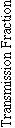 node.19 This requires a total of S integers, each in the range 0 to S. A node can not have itself as a receiver. The number of
distinct network configurations is then SS. For 25 sensors, there are 8.9(10)34 possible network configurations.
node.19 This requires a total of S integers, each in the range 0 to S. A node can not have itself as a receiver. The number of
distinct network configurations is then SS. For 25 sensors, there are 8.9(10)34 possible network configurations.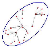 The shortest-path algorithm was used to generate the network that minimizes the transmission losses from each node to the
collection point. The shortest-path tree algorithm minimizes the sum of the weights associated with all edges in the paths
from any node to the root node. The algorithm can be used by equating the weight associated with an edge to the natural log
of the inverse of the transmission fraction. Then minimizing the sum of the weights along a path is equivalent to maximizing
the total transmission fraction along the path. The shortest-path network is shown in Fig 4, where the sensors have the same
locations as in Fig. 2. For this network configuration, the average message loss fraction is 0.03185, which is representative of
25 sensors in a 10 by 20 km elliptical area, where the transmission range scale is 5 km.
The shortest-path algorithm was used to generate the network that minimizes the transmission losses from each node to the
collection point. The shortest-path tree algorithm minimizes the sum of the weights associated with all edges in the paths
from any node to the root node. The algorithm can be used by equating the weight associated with an edge to the natural log
of the inverse of the transmission fraction. Then minimizing the sum of the weights along a path is equivalent to maximizing
the total transmission fraction along the path. The shortest-path network is shown in Fig 4, where the sensors have the same
locations as in Fig. 2. For this network configuration, the average message loss fraction is 0.03185, which is representative of
25 sensors in a 10 by 20 km elliptical area, where the transmission range scale is 5 km. Number of Evaluations
 Number of Evaluations